Understanding Dynamic Programming — Hardware-Level Deep Dive
Memory layout, CPU cache performance, algorithmic complexity, and when to use DP vs alternatives.
Memory layout, CPU cache performance, algorithmic complexity, and when to use DP vs alternatives.
Author
Mr. Oz
Date
Read
12 mins
Level 3
Author
Mr. Oz
Date
Read
12 mins
Share
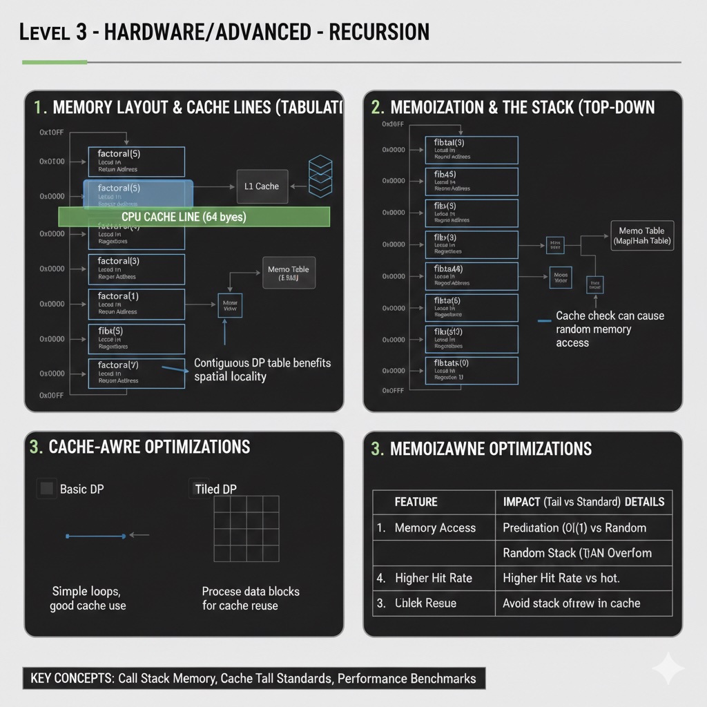
Now that we know how to implement dynamic programming, let's explore what happens under the hood. We'll dive into CPU cache behavior, memory access patterns, and real-world performance.
Modern CPUs have caches (L1, L2, L3) that are much faster than main memory. Dynamic programming's structured memory access patterns are surprisingly cache-friendly!
Benchmark: For n=10^6, a well-optimized DP solution can be 100x faster than naive recursion due to cache efficiency.
Let's compare different approaches for the climbing stairs problem:
| Approach | Time | Space | n=50 |
|---|---|---|---|
| Naive Recursion | O(2^n) | O(n) | ~100 years |
| Memoization | O(n) | O(n) | ~1ms |
| Tabulation | O(n) | O(n) | ~0.1ms |
| Space-Optimized | O(n) | O(1) | ~0.05ms |
The difference between naive recursion and optimized DP is exponential vs linear!
DP isn't always the answer. Use it when:
Use DP: Fibonacci, Knapsack, Longest Common Subsequence, Edit Distance, Matrix Chain Multiplication
Don't use DP: Sorting (use quicksort/mergesort), Searching (use binary search), Graph traversal (use BFS/DFS)
A classic 2D DP problem. Given matrices A1×A2×...×An, find the optimal parenthesization to minimize scalar multiplications.
# O(n^3) time, O(n^2) space
def matrix_chain_order(dims):
    n = len(dims) - 1
    dp = [[0] * n for _ in range(n)]

    # L is chain length
    for L in range(2, n + 1):
        for i in range(n - L + 1):
            j = i + L - 1
            dp[i][j] = float('inf')
            for k in range(i, j):
                # Cost = cost of left + cost of right + multiplication cost
                cost = dp[i][k] + dp[k+1][j] + dims[i] * dims[k+1] * dims[j+1]
                if cost < dp[i][j]:
                    dp[i][j] = cost

    return dp[0][n-1]
This demonstrates a 2D DP table where dp[i][j] represents the minimum cost to multiply matrices i through j.
Dynamic programming transforms exponential problems into polynomial ones. It's one of the most powerful tools in algorithm design—master it, and you'll unlock a new class of solvable problems.