Understanding Tree Construction: Implementation Guide
Turn the blueprint-and-inventory concept from Level 1 into production-ready code. We cover Python, Java, and C++ implementations with hashmap optimization and common pitfalls.
Turn the blueprint-and-inventory concept from Level 1 into production-ready code. We cover Python, Java, and C++ implementations with hashmap optimization and common pitfalls.
Author
Mr. Oz
Date
Read
8 mins
Level 2
Author
Mr. Oz
Date
Read
8 mins
Share
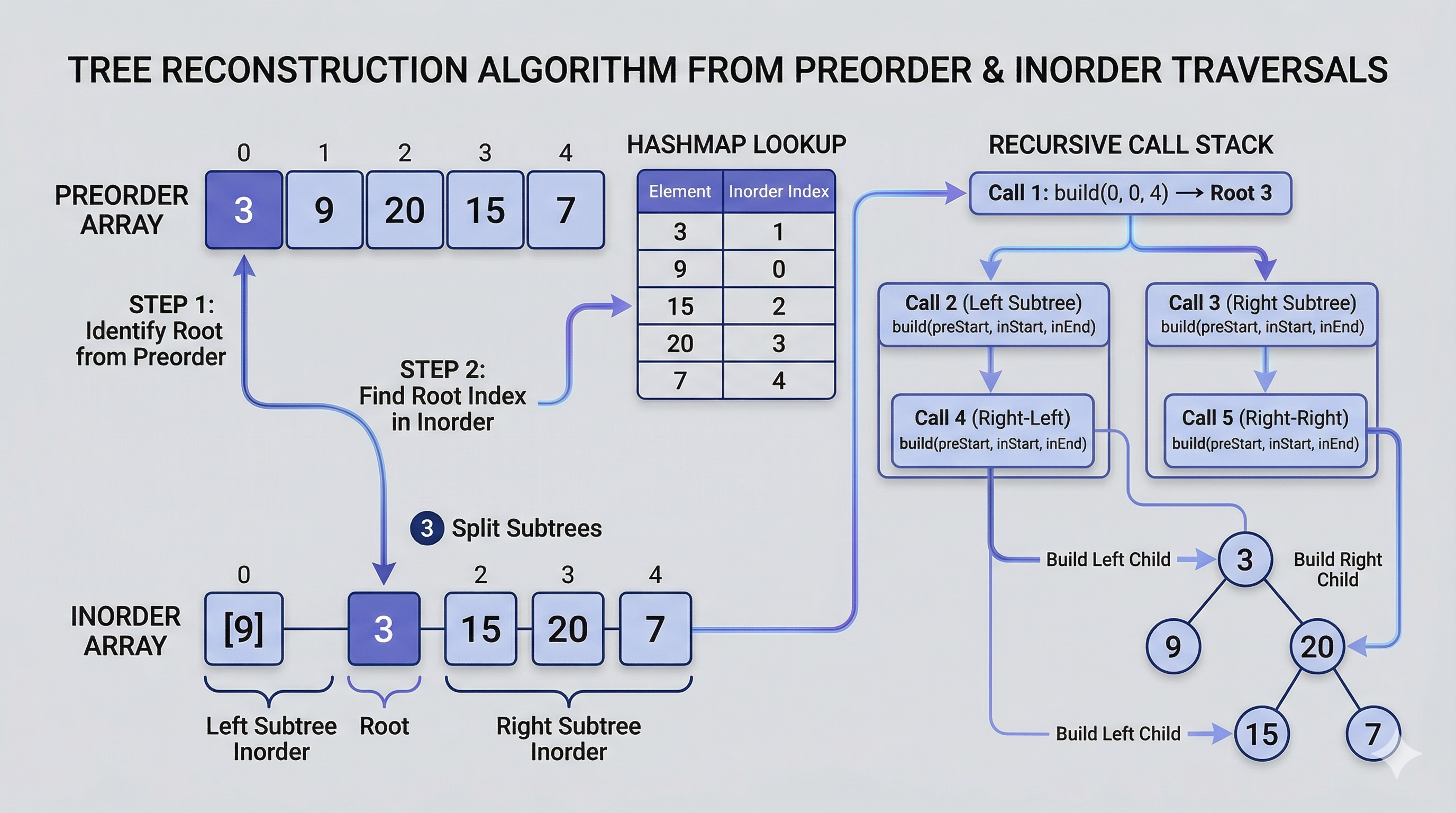
In Level 1, we learned the core idea: preorder gives us the root, inorder tells us where the left and right subtrees begin and end. Now it is time to translate that intuition into clean, efficient code across three major languages.
Every implementation starts with a tree node. The node holds a value and pointers to its left and right children. This is the universal foundation across all three languages.
# Python
class TreeNode:
    def __init__(self, val=0, left=None, right=None):
        self.val = val
        self.left = left
        self.right = right

// Java
class TreeNode {
    int val;
    TreeNode left;
    TreeNode right;
    TreeNode(int val) { this.val = val; }
}

// C++
struct TreeNode {
    int val;
    TreeNode *left;
    TreeNode *right;
    TreeNode(int x) : val(x), left(nullptr), right(nullptr) {}
};
This is the professional pattern. Notice how each language handles optional pointers differently:
Python uses None,
Java defaults to null,
and C++ uses nullptr.
The key optimization is building a hashmap that maps each inorder value to its index. This converts every root lookup from O(n) linear scan to O(1) constant-time access.
class Solution:
    def buildTree(self, preorder: list[int], inorder: list[int]) -> TreeNode:
        inorder_map = {val: i for i, val in enumerate(inorder)}
        pre_idx = 0

        def build(left: int, right: int) -> TreeNode:
            nonlocal pre_idx
            if left > right:
                return None

            root_val = preorder[pre_idx]
            pre_idx += 1
            root = TreeNode(root_val)

            mid = inorder_map[root_val]
            root.left = build(left, mid - 1)
            root.right = build(mid + 1, right)
            return root

        return build(0, len(inorder) - 1)
Line-by-line breakdown:
left and right define the current inorder boundary.The preorder index pointer technique avoids array slicing. Instead of creating new sublists (which costs O(n) per call), we pass boundary indices and reuse the original arrays. This reduces total time from O(n²) to O(n).
class Solution {
    private int preIdx = 0;
    private Map<Integer, Integer> inorderMap = new HashMap<>();

    public TreeNode buildTree(int[] preorder, int[] inorder) {
        for (int i = 0; i < inorder.length; i++) {
            inorderMap.put(inorder[i], i);
        }
        return build(preorder, 0, inorder.length - 1);
    }

    private TreeNode build(int[] preorder, int left, int right) {
        if (left > right) return null;

        int rootVal = preorder[preIdx++];
        TreeNode root = new TreeNode(rootVal);
        int mid = inorderMap.get(rootVal);

        root.left = build(preorder, left, mid - 1);
        root.right = build(preorder, mid + 1, right);
        return root;
    }
}
The Java version mirrors the Python logic exactly. The hashmap is stored as an instance field,
and the preorder index is an integer member that increments with each recursive call. Java's
HashMap provides O(1) average lookup.
class Solution {
    int preIdx = 0;
    unordered_map<int, int> inorderMap;

public:
    TreeNode* buildTree(vector<int>& preorder, vector<int>& inorder) {
        for (int i = 0; i < inorder.size(); i++)
            inorderMap[inorder[i]] = i;
        return build(preorder, 0, inorder.size() - 1);
    }

private:
    TreeNode* build(vector<int>& preorder, int left, int right) {
        if (left > right) return nullptr;

        int rootVal = preorder[preIdx++];
        TreeNode* root = new TreeNode(rootVal);
        int mid = inorderMap[rootVal];

        root->left = build(preorder, left, mid - 1);
        root->right = build(preorder, mid + 1, right);
        return root;
    }
};
C++ uses unordered_map for the same O(1) lookup.
Pass the preorder vector by reference to avoid copying. Remember that in C++ you manage memory manually —
in a production system you would want smart pointers or a destructor to free nodes.
mid instead of
mid - 1 for the left boundary or
mid + 1 for the right.
The root itself is excluded from both subtrees.| Operation | Time | Space |
|---|---|---|
| Build hashmap | O(n) | O(n) |
| Root lookup | O(1) | O(1) |
| Full construction | O(n) | O(n) + O(h) |
| Validate inputs | O(n) | O(n) |
Ready for more?
Level 1

Learn how binary trees can be reconstructed from traversals using a building blueprint analogy.
Author
Mr. Oz
Duration
5 mins
Level 2
Step-by-step code implementation in Python, Java, and C++ with hashmap optimization and common pitfalls.
Author
Mr. Oz
Duration
8 mins
Level 3

Memory layout, CPU cache, iterative construction, and real-world use cases in compilers and parsers.
Author
Mr. Oz
Duration
12 mins