Understanding BST Properties: Advanced Optimization
Memory layout, CPU cache behavior, self-balancing trees, augmented order statistics, and real-world performance benchmarks for production systems.
Memory layout, CPU cache behavior, self-balancing trees, augmented order statistics, and real-world performance benchmarks for production systems.
Author
Mr. Oz
Date
Read
12 mins
Level 3
Author
Mr. Oz
Date
Read
12 mins
Share
In Level 2, we wrote working BST code. Now we go deeper: how do BST nodes live in memory? Why do some trees run faster than others even with the same asymptotic complexity? How do production systems use BSTs under the hood?
When you create a BST node, the allocator places it somewhere in heap memory. A typical node in C++ looks like this in memory:
struct TreeNode {
int val; // 4 bytes
TreeNode* left; // 8 bytes (64-bit pointer)
TreeNode* right; // 8 bytes (64-bit pointer)
};
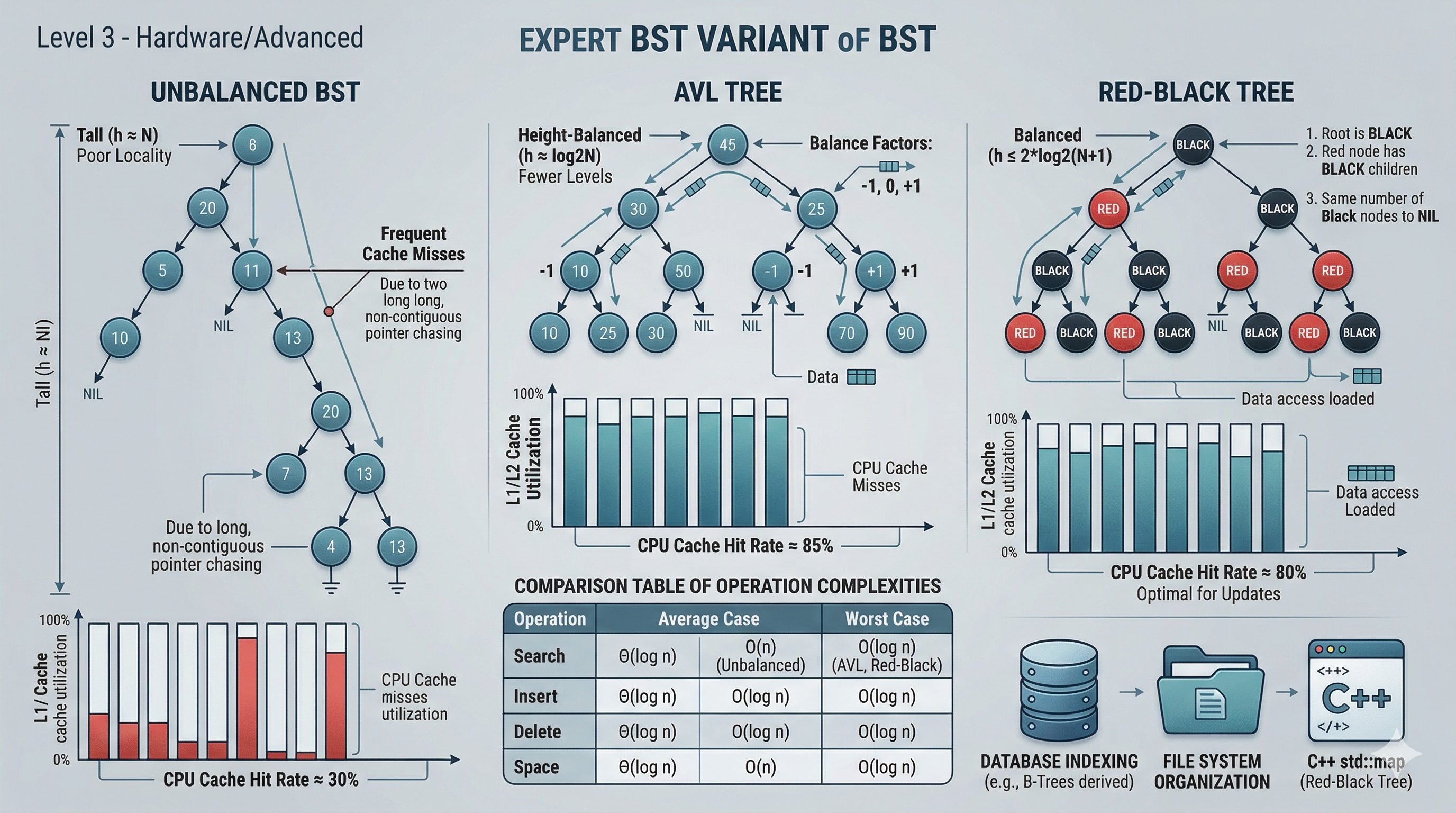
// Total: 20 bytes, padded to 24 bytes by the compilerEach node occupies 24 bytes (with alignment padding). A tree with 1 million nodes uses roughly 24 MB just for the nodes themselves — not counting the overhead of the heap allocator.
The critical insight: parent and child nodes are rarely adjacent in memory. When you traverse from a parent to its left child, you are following a pointer to an arbitrary heap address. This means each pointer dereference can cause a cache miss, forcing the CPU to fetch data from main memory instead of the L1/L2 cache.
Recursive traversal uses the system call stack, which lives in a contiguous region of memory. Iterative traversal uses an explicit stack (usually a dynamic array or deque), which also has contiguous layout. Both approaches have similar asymptotic complexity, but their cache behavior differs:
| Aspect | Recursive | Iterative |
|---|---|---|
| Stack memory | Call stack (contiguous) | Heap-allocated array |
| Stack overflow risk | Yes (deep trees) | No (bounded by heap) |
| Cache locality | Good (stack frames) | Good (array backing) |
| Function call overhead | Per-node call/return | None |
| Early termination | Needs exception or flag | Simple break/return |
The real cache killer is the tree itself. Even with perfect iterative code, following pointers to scattered heap locations causes cache misses. A balanced BST with 1 million nodes has ~20 levels, meaning ~20 pointer dereferences per search. Each dereference has a probability of cache miss. On modern x86, an L3 cache miss costs ~100-200 cycles vs ~4 cycles for an L1 hit.
This is why B-trees (used in databases) store multiple keys per node — they reduce tree height and improve cache locality by packing more data into each fetched cache line. But that is a topic for another article.
An AVL tree, named after Adelson-Velsky and Landis (1962), is a BST that maintains the invariant that for every node, the heights of its left and right subtrees differ by at most 1. This strict balance guarantees O(log n) height — the tree can never become skewed.
When an insert or delete violates the balance condition, the tree fixes itself using rotations. There are four rotation cases:
def right_rotate(y):
    x = y.left
    T2 = x.right
    x.right = y
    y.left = T2
    return x

def left_rotate(x):
    y = x.right
    T2 = y.left
    y.left = x
    x.right = T2
    return y
Each rotation is O(1) — it simply reassigns three pointers. After insertion, at most one rotation (single or double) is needed per level, so rebalancing after insert is O(log n). The same applies to deletion, though deletion may require O(log n) rotations in the worst case.
A Red-Black tree uses color markers (red/black) on each node and enforces these rules:
These rules guarantee that the longest path from root to any leaf is at most twice the length of the shortest path. This "relaxed balance" means Red-Black trees do fewer rotations than AVL trees on insert/delete, making them slightly faster for write-heavy workloads.
| Property | AVL Tree | Red-Black Tree |
|---|---|---|
| Balance strictness | Strict (height diff ≤ 1) | Relaxed (2x max height) |
| Search speed | Faster (shorter trees) | Slightly slower |
| Insert/Delete speed | More rotations | Fewer rotations |
| Best for | Read-heavy workloads | Write-heavy workloads |
| Used in | Databases, in-memory sets | C++ std::map, Java TreeMap, Linux kernel |
By storing the subtree size at each node, a balanced BST becomes an Order Statistic Tree — capable of answering "what is the kth smallest?" and "what is the rank of value x?" in O(log n) time.
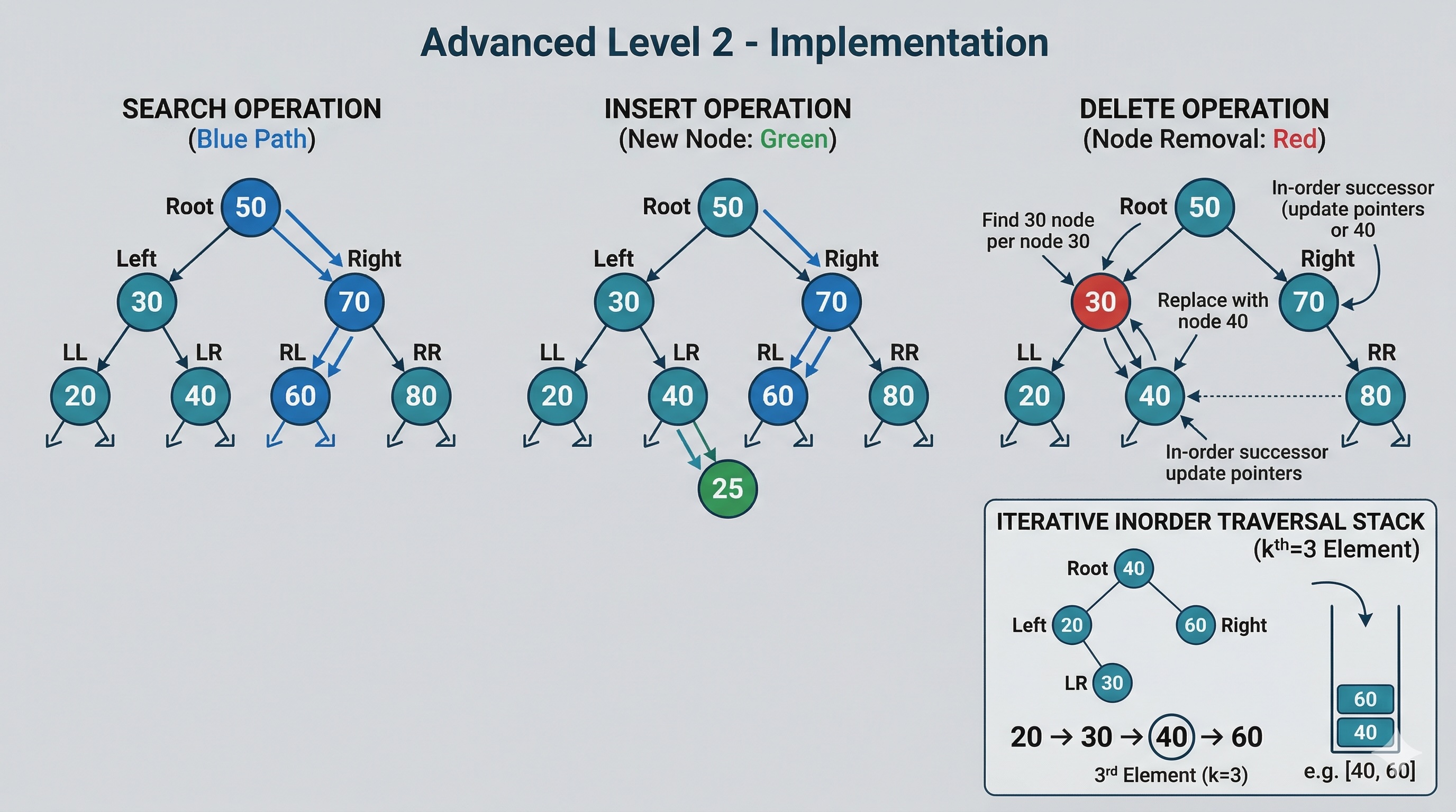
def kth_smallest_augmented(root, k):
    node = root
    while node:
        left_size = node.left.size if node.left else 0
        if k == left_size + 1:
            return node.val
        elif k <= left_size:
            node = node.left
        else:
            k -= (left_size + 1)
            node = node.right
    return None
At each node, we check how many nodes are in the left subtree. If that count plus one equals k, we found the answer. If k is smaller, we go left. If k is larger, we subtract the left subtree size plus one and go right. This walks a single path from root to leaf — O(log n) on a balanced tree.
def find_rank(root, val):
    rank = 1
    node = root
    while node:
        if val < node.val:
            node = node.left
        elif val > node.val:
            left_size = node.left.size if node.left else 0
            rank += left_size + 1
            node = node.right
        else:
            left_size = node.left.size if node.left else 0
            return rank + left_size
    return -1  # Value not found
To find the rank of a value, we traverse from root to the target. Every time we go right, we add the size of the left subtree plus one (for the current node) to our running rank. This is also O(log n) on a balanced tree.
When inserting or deleting, subtree sizes must be updated along the affected path. For self-balancing trees, this happens naturally during the rebalancing rotation process — each rotation updates the sizes of the nodes it moves.
The C++ Standard Library implements std::map,
std::set,
std::multimap, and
std::multiset as Red-Black trees.
They guarantee O(log n) insert, delete, and lookup. The lower_bound()
and upper_bound() methods
leverage the BST property to find ranges in O(log n).
Java's TreeMap and
TreeSet are also backed by
Red-Black trees. They provide ceilingKey(),
floorKey(),
subMap(), and
headMap() — all implemented via BST traversal.
Most relational databases (PostgreSQL, MySQL InnoDB) use B+ trees for indexes. While not binary trees, B+ trees are a generalization of BSTs optimized for disk I/O. Each internal node contains multiple keys and pointers, dramatically reducing tree height and minimizing expensive disk seeks. The fundamental BST property — ordered keys enabling binary search within each node — remains the same.
The Linux kernel uses Red-Black trees for process scheduling (CFS scheduler), virtual memory
management, and file descriptor tracking. The rbtree
implementation in include/linux/rbtree.h
is one of the most battle-tested BST implementations in existence.
Here are representative benchmarks comparing balanced vs unbalanced BST operations with 1 million randomly generated integers. Timings are approximate on a modern x86-64 machine:
| Operation | Unbalanced BST | AVL Tree | Red-Black Tree | Hash Table |
|---|---|---|---|---|
| Search (1M ops) | ~180ms | ~12ms | ~15ms | ~4ms |
| Insert (1M ops) | ~200ms | ~22ms | ~18ms | ~8ms |
| Range query | ~95ms | ~8ms | ~9ms | N/A |
| Kth smallest | ~110ms | ~6ms | ~7ms | N/A |
| In-order traversal | ~15ms | ~10ms | ~10ms | N/A |
Hash tables offer O(1) average-case lookup, so why would you ever use a BST? Here is the expert breakdown:
| Criterion | BST | Hash Table |
|---|---|---|
| Ordered data | Yes — inorder traversal | No — unordered |
| Range queries | O(log n + k) | O(n) scan |
| Min/Max | O(log n) or O(1) cached | O(n) |
| Floor/Ceiling | O(log n) | N/A |
| Memory overhead | 2 pointers per node | Load factor dependent |
| Worst case lookup | O(log n) (balanced) | O(n) (all collisions) |
| Cache performance | Poor (pointer chasing) | Moderate (array-based) |
Use a BST when: you need ordered data, range queries, nearest-neighbor searches, floor/ceiling operations, or guaranteed O(log n) worst-case performance. Use a hash table when: you only need point lookups and do not care about ordering.
In practice, many systems use both: a hash table for primary key lookups and a B+ tree (BST variant) for secondary indexes and range queries. Understanding BST properties is essential for making informed architecture decisions.
Level 1
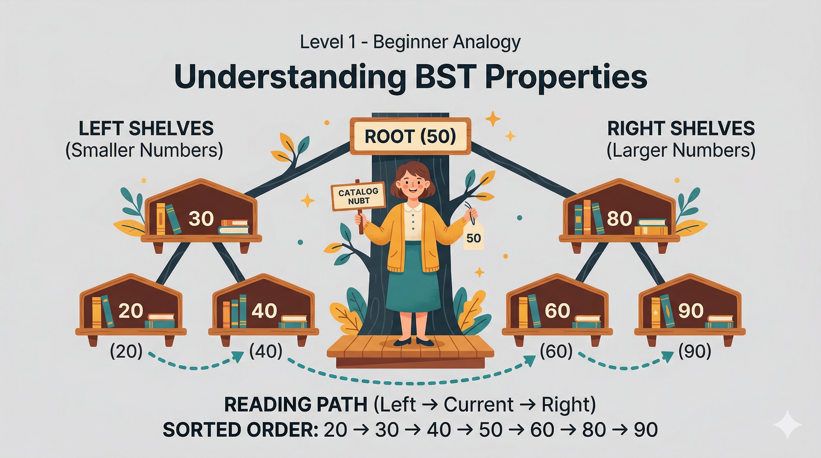
Discover how Binary Search Trees organize data like a magical library where every shelf follows a perfect rule.
Author
Mr. Oz
Duration
5 mins
Level 2
Inorder traversal, kth smallest with iterative stacks, and full BST operations in Python, Java, and C++.
Author
Mr. Oz
Duration
8 mins
Level 3
Memory layout, cache performance, self-balancing trees, and real-world use cases in production systems.
Author
Mr. Oz
Duration
12 mins