Understanding Binary Search Trees — Level 3
Expert-level optimization: master balancing algorithms, explore AVL and Red-Black trees, and understand memory layout implications for production-grade performance.
Expert-level optimization: master balancing algorithms, explore AVL and Red-Black trees, and understand memory layout implications for production-grade performance.
Author
Mr. Oz
Date
Read
12 mins
Level 3
Author
Mr. Oz
Date
Read
12 mins
Share
In Levels 1 and 2, we understood what BSTs are and how to implement them. Now we'll explore why naive BSTs fail in production and how balanced variants solve these problems.
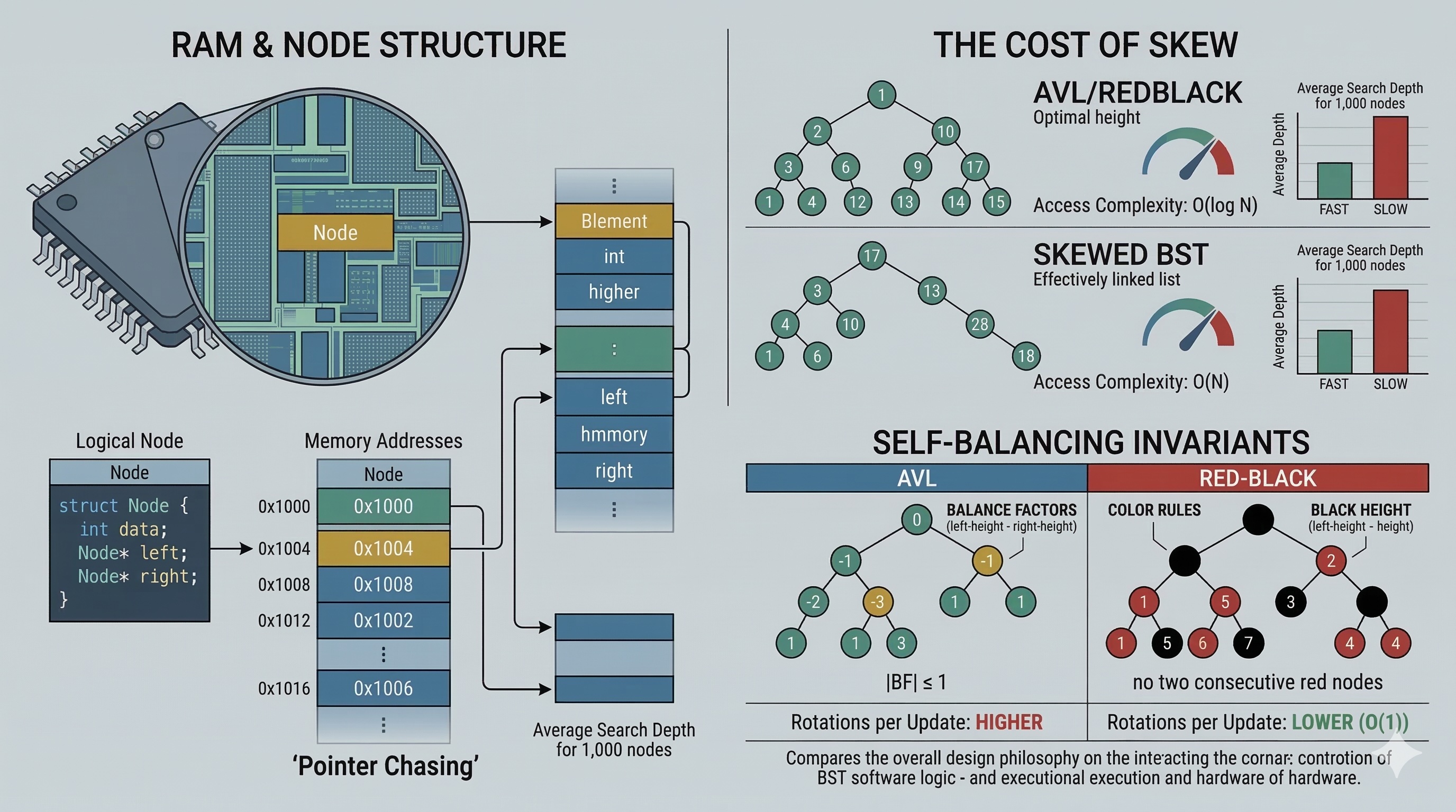
A naive BST has a critical flaw: its performance depends entirely on insertion order. Insert elements in sorted order, and you get a linked list, not a tree.
# Inserting 1, 2, 3, 4, 5 in order:
1
\
2
\
3
\
4
\
5
# Search time: O(n) — no better than linear search!
Real-world impact: If you're building a BST from sorted database records, your "O(log n)" operations become O(n), potentially causing production outages.
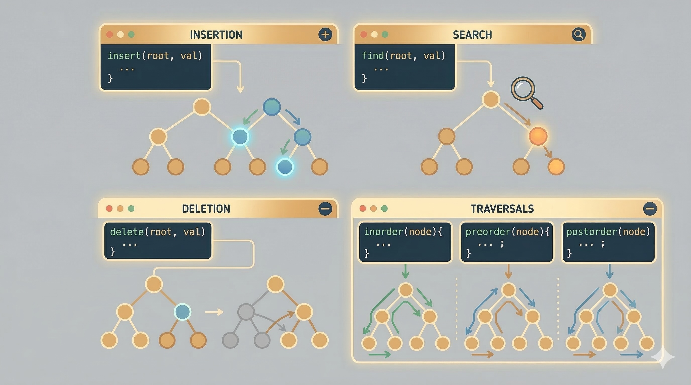
Self-balancing trees detect when they're becoming unbalanced and automatically restructure. Two dominant approaches exist:
AVL trees maintain balance through four rotation types. The "balance factor" (height(left) - height(right)) determines which rotation to apply:
# Calculate balance factor
def get_balance(node):
if not node: return 0
return height(node.left) - height(node.right)
# Balance factor > 1: left-heavy (rotate right)
# Balance factor < -1: right-heavy (rotate left)
Before:
x
\
y
After:
y
/
x
Before:
z
/
y
After:
y
\
z
Double rotations (Left-Right, Right-Left) handle cases where a single rotation doesn't fix the imbalance.
Red-Black trees use node colors to enforce balance. The rules are:
These rules guarantee that the longest path is at most twice the shortest path, ensuring O(log n) operations.
# Insert fixup pseudocode
def insert_fixup(root, node):
while node.parent is RED:
if parent is left child:
uncle = node.parent.parent.right
if uncle is RED:
# Case 1: Recolor
node.parent = BLACK
uncle = BLACK
node.parent.parent = RED
node = node.parent.parent
else:
# Cases 2 & 3: Rotate
...
root.color = BLACK
BSTs have a hidden performance cost: pointer chasing. Each node is typically allocated separately on the heap, causing cache misses.
| Data Structure | Cache Locality | Why |
|---|---|---|
| Array | Excellent | Contiguous memory |
| BST (naive) | Poor | Random heap allocations |
| B-Tree | Good | Multiple keys per node |
Practical tip: For performance-critical code, consider B-trees or Eytzinger layout arrays instead of pointer-based BSTs.
std::map —
Uses Red-Black tree; guarantees O(log n) operations
TreeMap —
Red-Black tree implementation for sorted key-value storage
bisect —
Uses binary search on arrays (not BSTs) for better cache performance
| Scenario | Best Choice |
|---|---|
| Static sorted data, many lookups | Sorted array + binary search |
| Dynamic data, many reads | AVL tree |
| Dynamic data, balanced read/write | Red-Black tree |
| Disk-based storage | B+ tree |
| In-memory, cache-sensitive | B-tree or Eytzinger array |
# Search performance (nanoseconds per operation)
Sorted array (binary search): ~15ns
AVL tree (balanced): ~45ns
Red-Black tree: ~50ns
Naive BST (worst case): ~450ns (10× slower!)
# Insert performance
AVL tree: ~80ns
Red-Black tree: ~60ns
Benchmarks on Intel i7, single-threaded. Your results may vary.
Completed all 3 levels?
You now understand BSTs from analogy to production optimization.
Level 1

Learn the fundamentals of BSTs through an engaging magical library analogy.
Author
Mr. Oz
Duration
5 mins
Level 2
Implementation details, insertion, search, deletion, and traversal operations.
Author
Mr. Oz
Duration
8 mins
Level 3
Balancing techniques, AVL trees, Red-Black trees, and performance optimization.
Author
Mr. Oz
Duration
12 mins